Fighting the regression

THE CHALLENGE: REGRESSION TO THE MEAN

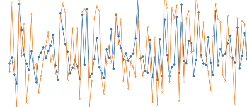
Over the last few weeks, I carved out time to work on a small time series model, aiming to predict data usage. The journey began with a core challenge: the data was highly skewed and concentrated, seemingly random within a tight normal range. Extreme density around the mean value turned model building into a battle to justify its value, as even basic statistics – like averaging over months – seemed almost as effective. In short, regression to the mean was our enemy, as the data seemed devoid of useful variability.

PRE-PROCESSING FOR SIGNAL

As with any ML problem, pre-processing was vital, and here I learned a few key lessons. Due to the data’s commercial sensitivity, I can’t reveal specifics, but the extreme density around the mean value meant that simply sampling data to dilute the concentration didn’t help. It remained challenging for the model to capture any pattern.

Given a 24-month time span, I experimented with windowing techniques, such as rolling averages and peak-value extractions. A major decision lay in defining the target value. Initially, I tried using a derived combination of two columns to create a single normalized number for deployment. Unfortunately, this didn’t capture the effect we were hoping for as well as using an absolute column value. Eventually, I settled on using an LSTM and applying rolling averages and peak values within specific windows, which enabled some capture of temporal patterns.

The takeaway here? Don’t settle too early on a target, assuming domain-normalized values are the only option. Sometimes, a straightforward approach can yield more insight.

WHICH MODEL TO USE?

I’m writing this before any production deployment, while the pain of trial and error is still fresh. The model itself may still evolve from the current LSTM. Initially, I tried an XGBoost hybrid for its robustness with sparse data, but it, too, fell prey to the narrow range of predictions. An ensemble architecture followed, designed to handle each main data area individually, but it also struggled with the tight range.

An early attempt with a transformer model didn’t yield much, although since then, I’ve refined the training data, so a revisit may be worth it. For now, the LSTM’s ability to highlight temporal patterns, combined with engineered features, has managed to surface some signals in the data.

CUSTOM LOSS FUNCTIONS

For a couple of days, I focused on custom loss functions, aiming to pull predictions away from the mean. The goal was to exaggerate variance, capturing spikes or dips that generic loss functions were ignoring. Below is an early iteration of this work, where predictions are “stretched” from the mean. I also experimented with a quantile loss function, though the result remained underwhelming.

class WeightedMSELoss(nn.Module):

def __init__(self, base_weight=1.0, prob_weight=2.0, stretch_factor=1.2):
    super(WeightedMSELoss, self).__init__()
    self.base_weight = base_weight
    self.prob_weight = prob_weight
    self.stretch_factor = stretch_factor

def forward(self, predictions, targets, temporal_weights):
    mean_pred = torch.mean(predictions)
    mean_target = torch.mean(targets)
    stretched_preds = mean_pred + (predictions - mean_pred) * self.stretch_factor
    weights = self.base_weight + (temporal_weights * self.prob_weight)
    deviation_weight = 1.0 + torch.abs(targets - mean_target) / mean_target
    weights = weights * deviation_weight
    return torch.mean(weights * (stretched_preds - targets) ** 2)

OPTIMIZING TRAINING EPOCHS

With the development pipeline in place, I focused on training configurations. The model generalized well early on, but I assumed lower loss scores meant more training was beneficial. Here’s where I went wrong. Post-analysis showed I was overtraining; five epochs sufficed! This underscored the importance of ongoing evaluation instead of assuming that lower loss always equals better predictions.

RESULTS AND INSIGHTS

A final adjustment involved grouping predictions, which helped reduce noise in practical applications and better aligned with the use case. Visualizing grouped predictions against actual results, with standard deviation bands in the background, provided valuable insights into the model’s reactions. However, without a set of ‘evals’ for accepted prediction ranges, further fine-tuning will likely be needed. Running more experiments programmatically will help expose model weaknesses.